Effective quasi-harmonic potential

This example shows how to fit the effective quasi-harmonic potential as a function of volume and temperature.

import numpy as np
from ase.build import bulk
from tensorpotential.calculator import grace_fm

from directupsampling.calculators.emt import EMT
from directupsampling.effqh.effqh import EffQH
from directupsampling.plot_tools import plot
from directupsampling.sampling import GridSampler

[tensorpotential] Info: Environment variable TF_USE_LEGACY_KERAS is automatically set to '1'.
WARNING:tensorflow:UserWarning: enabling the new type promotion must happen at the beginning of the program. Please ensure no TF APIs have been used yet.
WARNING:tensorflow:UserWarning: enabling the new type promotion must happen at the beginning of the program. Please ensure no TF APIs have been used yet.
WARNING:tensorflow:UserWarning: enabling the new type promotion must happen at the beginning of the program. Please ensure no TF APIs have been used yet.
WARNING:tensorflow:UserWarning: enabling the new type promotion must happen at the beginning of the program. Please ensure no TF APIs have been used yet.
WARNING:tensorflow:UserWarning: enabling the new type promotion must happen at the beginning of the program. Please ensure no TF APIs have been used yet.

Make the initial ASE Atoms object.

atoms = bulk("Al", "fcc", cubic=True) * 3

Make two calculators. The first one is a light-weight calculator to sample MD trajectories. The second one is an accurate calculator to compute forces on atoms. The accurate calculator is typically a DFT calculator. In this example, we intead use a GRACE foundation model.

atoms.calc = EMT()
calc_dft = grace_fm("GRACE-1L-OMAT")

Using cached GRACE model from /root/.cache/grace/GRACE-1L-OMAT
Model license: Academic Software License

Define a volume-temperature grid using a GridSampler.

temperature = 20.0  # in K
grid_fqh = [(v, temperature) for v in np.linspace(15.0, 18.0, 7)]
effqh_sampler = GridSampler(atoms, grid_fqh)

Run MD calculations. For a relatively light-weight calculator, we can run directly calculate_with. For a DFT calculator, it may be more convenient to first make input files using write_folders, run DFT calculations in these folders, and then collect the results using read_folders.

effqh_sampler.sample_snapshots(30)
snapshots_for_effqh = effqh_sampler.calculate_with(calc_dft)
# effqh_sampler.write_folders(
#     root_path="./calcs",
#     joblist_file="./jobList",
#     calc=std_dft,
# )
# Run DFT calculations in the folders.
# snapshots_for_effqh = GridSampler.read_folders("./calcs").snapshot_container

/usr/local/lib/python3.12/site-packages/ase/md/velocitydistribution.py:147: FutureWarning: `communicator` has been deprecated since ASE 3.26.0 and will be removed in ASE 3.27.0. Use `comm` instead.
  warnings.warn(msg, FutureWarning)
/usr/local/lib/python3.12/site-packages/ase/md/velocitydistribution.py:154: FutureWarning: `comm=="serial"` has been deprecated since ASE 3.26.0 and will be removed in ASE 3.27.0. Use `comm=DummyMPI()` instead.
  warnings.warn(msg, FutureWarning)

Fit the effective harmonic potential as a function of volume and temperature.

effqh = EffQH(atoms, fit_order=3)
effqh.fit_snapshots(snapshots_for_effqh, method="least-squares")
effqh.write_fc_fit("effqh_force_constants_fit.hdf5")

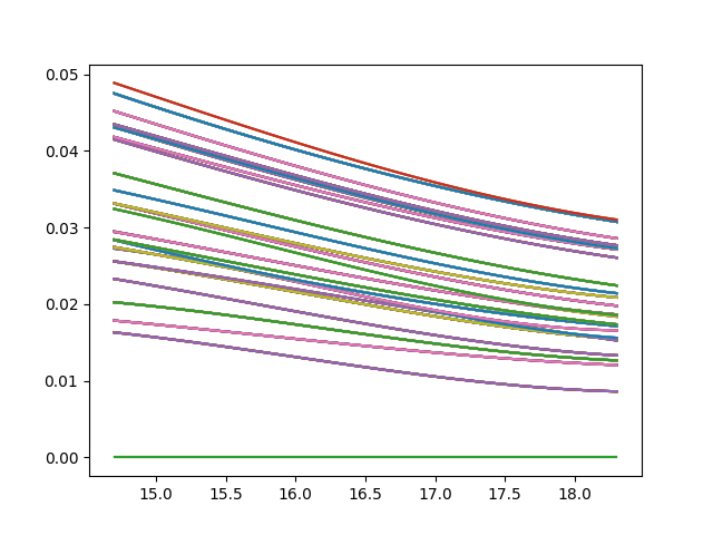
Check the quasi-harmonic frequencies.

plot(effqh.exact_phonons).show()